As of today, I have been programming for approximately 7 years. I hold a MSc. in Social and Econmic Data Analysis. I have written code in R, Python, C, Java, Javascript, HTML, CSS. I have numerous other programming-related skills. Still, I regularly get bitten in the a** when writing code. Quite often it has something to do with checking my assumptions. Today was an excellent example of this, so let me tell you a story…1
The original problem
I have written about my Spotify Liked Songs playlist in the past. Nowadays, I often go to my Liked Songs playlist to listen to my new favorite songs. However, while I enjoy the songs, I find it a slightly annoying that they’re always in the same order. Of course, I could (and have) enable “shuffle” but that means that I also get random songs from 1-2 years thrown in that I probably don’t enjoy as much anymore.
Given this - very privileged - “problem”, I thought: “mmhhh, I could fix that with the API probably.” For example, only take the last songs I have liked in the last few months and reorder them randomly. That should be easy, right? Well well well… Yes - if you keep it simple - and no - if you try to be particularly clever and fail to check your assumptions.
Getting the data
Ok, let’s get the tracks (code mostly hidden because it is literally copy-pasted from the other post):
Show code
# spotify api package
library(spotifyr)
# usual suspects
library(dplyr)
library(purrr)
library(readr)
library(ggplot2)
library(tidyr)
library(forcats)
# for my own custom function to remove songs from playlist
library(httr)
library(usethis)
library(glue)

# spotify colors
spotify_green <- "#1DB954"
spotify_black <- "#191414"
# ggplot theme
source("../ggplot_theme.R")
my_theme <- theme_frie_codes()

my_spotify_theme <- function() {
  theme_frie_codes()+
  theme(plot.background = element_rect(fill = spotify_black),
        axis.ticks = element_line(color = "#FFFFFF"),
        axis.line = element_line(color = "#FFFFFF"),
        axis.text = element_text(color = "#FFFFFF"),
        axis.title = element_text(color = "#FFFFFF"))
}
theme_set(my_spotify_theme())
Show code
access_token <- spotifyr::get_spotify_access_token()
# get total number of saved tracks and calculate the offsets (can only get 50 tracks with a call)
meta <- spotifyr::get_my_saved_tracks(limit = 50, offset = 0, include_meta_info = TRUE)
total <- meta$total # total number of saved tracks
offsets <- seq(0, total + 50, 50)
# define function to get 50 saved tracks depending on offset
get_chunk <- function(offset) {
  new <- spotifyr::get_my_saved_tracks(limit = 50, offset = offset, include_meta_info = FALSE)
  usethis::ui_done(glue::glue("got from offset: {offset}"))
  return(new)
}
Let’s do some cleaning.
A short look when I added the songs (and having fun with ggplot theming):
Show code
all_tracks %>%
  ggplot(aes(x = added_at))+
  geom_histogram(fill = spotify_green, color = spotify_black)+
  scale_x_datetime(breaks = "6 months",date_labels = "%Y-%m")+
  theme(axis.text.x = element_text(angle = 90))+
  NULL
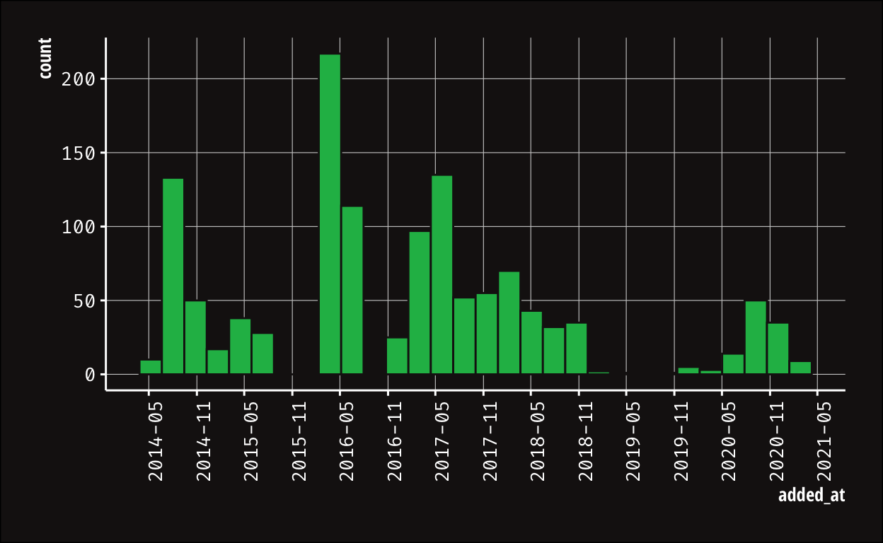
I should probably look at what happened in April 2016 but that’s the topic for another post.
The (failed) solution
Instead of only looking at the last weeks’ worth of liked songs, I decided to do the full Covid year, in honor of the upcoming (German) lockdown/pandemic anniversary which coincides with my “living in Berlin” anniversary… yey. 🎉 This also makes sense because my music taste does not evolve fast.
Quick check that I still like the songs that I added at the beginning of this time period2:
                                                  track.name
106 I Miss Having Sex But At Least I Don't Wanna Die Anymore
107                                  Watch What Happens Next
108                                            Asthma Attack
109                       Despacito (Featuring Daddy Yankee)
110                         death bed (coffee for your head)
111                               i wanna be your girlfriend
My original idea was to “unlike” the songs (as I have done in my other blog post) and like them again. This probably would’ve worked but I googled around and stumbled across “Reorder or Replace a Playlist’s Items”, which is implemented as a PUT on the playlists/{playlist_id}/tracks endpoint: https://api.spotify.com/v1/playlists/{playlist_id}/tracks3. I instantly focused on that because that would mean that I could keep the original added_at information - so much more elegant and cool!
⚠️ Here is obviously where things went wrong - can you guess what the problem might be? ⚠️
After procrastinating a little bit by looking at the genres of the artists4, I told myself “focus!” and so I did finally look at how I would implement this.
So you can pass three arguments to the endpoint:
range_start: “The position of the first item to be reordered.”range_length: “The amount of items to be reordered. Defaults to 1 if not set.” –> 1 in my case because I did not want to reorder “chunks” but individual songs.insert_before: “The position where the items should be inserted.”
So, I sampled the new positions (the old_pos was defined above in the data cleaning - Spotify conveniently returns the songs in the order you have added them, with the newest being the first row):
set.seed(123)
covid_tracks <- covid_tracks %>%
  mutate(old_pos = as.numeric(old_pos),
         new_pos = sample(old_pos, nrow(covid_tracks))) %>%
  arrange(new_pos) %>%
  select(old_pos, new_pos, everything())
Fun little plot to see that there is no significant correlation between the new and old position5:
Show code
ggplot(covid_tracks, aes(x = old_pos, y = new_pos))+
  geom_point(color = spotify_green)+
  geom_smooth(color = spotify_green)+
  labs(x = "old position in playlist", y = "new position in playlist")+
  theme(plot.background = element_rect(fill = spotify_black))
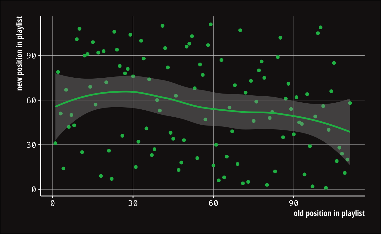
The main problem was that I had to make an API call for each of the 111 songs to reorder it to its new position. That meant that I could not just use the old_pos for the range_start because in the mean time it could have moved in the playlist as a result from the previous API calls. Does this make sense?
I spent a good 45 minutes thinking about this and came up with this hacky solution where I calculated a “correct factor” for each row6:
Show code
n_elements_to_correct_for <- function(old, new, df) {
  # we filter out those elements who will be moved before the current element
  # only if the old position of the other elements is larger than the current element, we have to "correct"
  correct_for <- df %>%
    filter(new_pos < new & old_pos > old)
  nrow(correct_for)
}

arg_df <- covid_tracks %>%
  select(old = old_pos, new = new_pos)

covid_tracks$moved_before_by_now <- pmap_dbl(arg_df, n_elements_to_correct_for, df = covid_tracks)
covid_tracks <- covid_tracks %>%
  mutate(find_pos = old_pos + moved_before_by_now)

covid_tracks %>%
  select(new_pos, old_pos, moved_before_by_now, find_pos) %>%
  arrange(new_pos) %>%
  head() %>%
  knitr::kable()
| new_pos | old_pos | moved_before_by_now | find_pos |
|---|---|---|---|
| 1 | 102 | 0 | 102 |
| 2 | 97 | 1 | 98 |
| 3 | 80 | 2 | 82 |
| 4 | 71 | 3 | 74 |
| 5 | 73 | 3 | 76 |
| 6 | 62 | 5 | 67 |
I even did a little test to convince me (and you) that this indeed is what is needed:
set.seed(356)
test_df <- tibble(new_pos = 1:10, old_pos = sample(1:10, 10))

arg_df <- test_df %>%
  select(old = old_pos, new = new_pos)

test_df$moved_before_by_now <- pmap_dbl(arg_df, n_elements_to_correct_for, df = test_df)
test_df <- test_df %>%
  mutate(find_pos = old_pos + moved_before_by_now)


test_df %>%
  arrange(new_pos)
# A tibble: 10 x 4
   new_pos old_pos moved_before_by_now find_pos
     <int>   <int>               <dbl>    <dbl>
 1       1      10                   0       10
 2       2       2                   1        3
 3       3       9                   1       10
 4       4       4                   2        6
 5       5       5                   2        7
 6       6       8                   2       10
 7       7       3                   5        8
 8       8       7                   3       10
 9       9       1                   8        9
10      10       6                   4       10
I then wanted to finally write the function to reorder the tracks given my new, fancy find_pos variable (for range_start). Given that this is not implemented in spotifyr, I copied my delete_ids function from my old blog post and adapted it:
# define function to reorder tracks
# cf https://developer.spotify.com/documentation/web-api/reference/#category-playlists
reorder_track <- function(find_pos) {
  httr::PUT(glue::glue("https://api.spotify.com/v1/playlists/{playlist_id}/tracks"),
            config =  httr::config(token = spotifyr::get_spotify_authorization_code()),
            query = list(range_start = find_pos, range_length = 1, insert_before = 0))
}
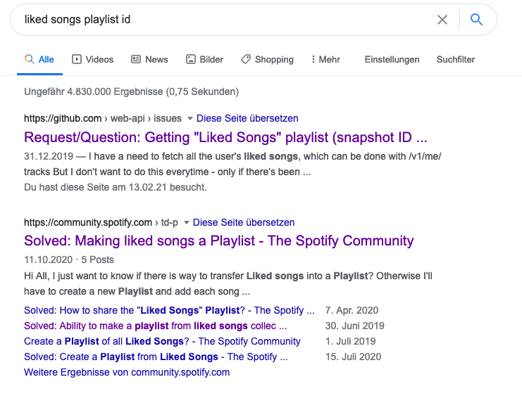
That’s when I went like “huh, what’s the playlist id of the liked songs playlist?”?
Well..turns out the liked songs playlist is not a playlist. Hence, it does not have a playlist id and you can’t reorder songs by using the API endpoint.7🤦
time –> 🗑
A simple Google confirmed it8:
At this point, I could have tried my original idea of removing and re-adding the songs by unliking and liking them again but there was already enough time and nerves wasted.
The end
Besides a bit of ggplot theme-ing and a very inefficent “algorithm”, there is nothing really to take away from this post except for the important lesson: Check your assumptions. Especially when you work with services / APIs / code that you have not written yourself. Our sophisticated internal image of our future code is often based on assumptions about the tools we’ll be using - whether that is an API, a programming framework like Shiny, a tool like Docker or R packages. So don’t be like me, have some patience and read the fine manual for a bit before you start coding like this:
Of course, you don’t have to read the documentation to bits and pieces every time before writing a line of code. Experimenting and exploring things on our own is a huge - and fun - part of programming. If I experiment with code, I try to timebox myself, e.g. I say “ok I will try this for x minutes by just fiddling around before I do some proper research”.
But sometimes, that’s not enough, especially if we are able to consistently make progress on our internal plan but one late step in it depends on an unchecked assumption (like me today). In those cases, we really have to step back early and dig into our assumptions so that we can…
…keep coding without being frustrated in the end. ❤️
Of course, I didn’t intend to write this post like this but now here we are.. 🤷.↩︎
The humor of this selection is not lost on me…↩︎
documentation here - you need to scroll a little, there is no deep link..↩︎
maybe follow-up post?↩︎
i mean..i used a random sampling method but idk…probability can be a bitch?↩︎
don’t bother understanding it unless you want to implement this for your Spotify… playlists↩︎
You can confirm this by going to your Spotify Desktop client and trying to reorder songs by drag-and-dropping them. It will work in your own playlists but not in the Liked Songs.↩︎
the “solution” from the second result is “make a playlist out of it and manually drag all the songs into it”↩︎